Description of Kohonen's Self-Organizing Map

Timo Honkela

Excerpt from "Self-Organizing Maps in Natural Language Processing".

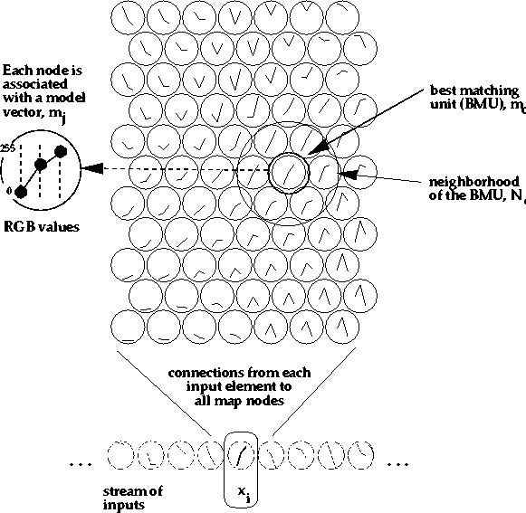
The basic Self-Organizing Map (SOM) can be visualized as a sheet-like neural-network array (see Figure 1), the cells (or nodes) of which become specifically tuned to various input signal patterns or classes of patterns in an orderly fashion. The learning process is competitive and unsupervised, meaning that no teacher is needed to define the correct output (or actually the cell into which the input is mapped) for an input. In the basic version, only one map node (winner) at a time is activated corresponding to each input. The locations of the responses in the array tend to become ordered in the learning process as if some meaningful nonlinear coordinate system for the different input features were being created over the network (Kohonen, 1995c).

The SOM was developed by Prof. Teuvo Kohonen in the early 1980s (Kohonen, 1981a, 1981b, 1981c, 1981d, 1982a, 1982b). The first application area of the SOM was speech recognition, or perhaps more accurately, speech-to-text transformation (Kohonen et al., 1984,Kohonen, 1988).

Self-Organizing Map algorithm

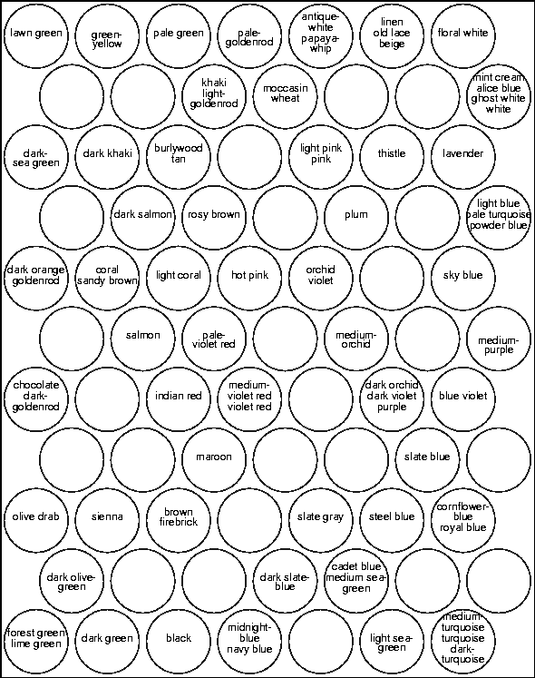
Assume that some sample data sets (such as in Table 1) have to be mapped onto the array depicted in Figure 1; the set of input samples is described by a real vector ${\bf x}(t) \in R^n$where t is the index of the sample, or the discrete-time coordinate. Each node i in the map contains a model vector ${\bf m}_i(t) \in R^n$,which has the same number of elements as the input vector ${\bf x}(t)$.

The stochastic SOM algorithm performs a regression process. Thereby, the initial values of the components of the model vector, ${\bf m}_i(t)$, may even be selected at random. In practical applications, however, the model vectors are more profitably initialized in some orderly fashion, e.g., along a two-dimensional subspace spanned by the two principal eigenvectors of the input data vectors (Kohonen, 1995c). Moreover, a batch version of the SOM algorithm may also be used (Kohonen, 1995c).

 

250 235 215 antique white

165 042 042 brown

222 184 135 burlywood

210 105 30 chocolate

255 127 80 coral

184 134 11 dark goldenrod

189 183 107 dark khaki

255 140 dark orange

233 150 122 dark salmon

... ... ... ...

Any input item is thought to be mapped into the location, the ${\bf m}_i(t)$ of which matches best with ${\bf x}(t)$ in some metric. The self-organizing algorithm creates the ordered mapping as a repetition of the following basic tasks:

1.

An input vector ${\bf x}(t)$is compared with all the model vectors ${\bf m}_i(t)$. The best-matching unit (node) on the map, i.e., the node where the model vector is most similar to the input vector in some metric (e.g. Euclidean) is identified. This best matching unit is often called the winner.

2.

The model vectors of the winner and a number of its neighboring nodes in the array are changed towards the input vector according to the learning principle specified below.

  

Figure 1: The basic architecture of the Self-Organizing Map (SOM). The input x is fully connected to the array of map nodes which is most often and also in this illustration two-dimensional. Each map node, visualized as a circle on the grid, serves as a model, m_i, or to use another term, a prototype of a class of similar inputs. The line diagrams inside the circles denote the three RGB values of Table 1. For instance, the nodes on the lower left corner correspond to colors which have high values of all the components, i.e., red, green, and blue and therefore that corner contains very dark colors.

The basic idea in the SOM learning process is that, for each sample input vector ${\bf x}(t)$,the winner and the nodes in its neighborhood are changed closer to ${\bf x}(t)$ in the input data space. During the learning process, individual changes may be contradictory, but the net outcome in the process is that ordered values for the ${\bf m}_i(t)$emerge over the array. If the number of available input samples is restricted, the samples must be presented reiteratively to the SOM algorithm. 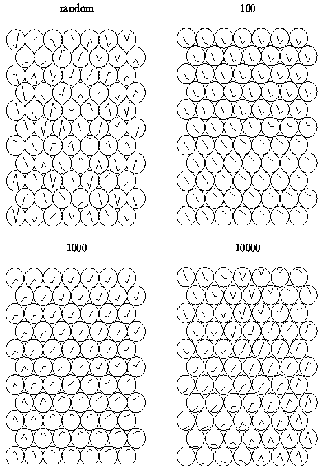The random initial state, two intermediate states, and the final map are shown in Figure 2.

  

Figure 2: An example of the first steps of the ordering process of a 7 times 11 map. Each circle corresponds to a map node. Inside the circle the model vector consisting of the three RGB values from Table 1 is visualized. The initial value of the learning step size, alpha₀, was 0.2 and the neighborhood width was initially 5. The value of both parameters decreased linearly during the learning process. The values above the nodes indicate the number of learning steps.

Adaptation of the model vectors in the learning process may take place according to the following equations:

${\bf m}_i(t+1)={\bf m}_i(t)+\alpha(t)[{\bf x}(t)-{\bf m}_i(t)] \mbox{\hspace{15 pt} for each } i \in N_c(t),$ (1)
${\bf m}_i(t+1)={\bf m}_i(t)$ otherwise,

where t is the discrete-time index of the variables, the factor $\alpha(t) \in [0,1]$ is a scalar that defines the relative size of the learning step, and N_c(t) specifies the neighborhood around the winner in the map array.

At the beginning of the learning process the radius of the neighborhood is fairly large, but it is made to shrink during learning. This ensures that the global order is obtained already at the beginning, whereas towards the end, as the radius gets smaller, the local corrections of the model vectors in the map will be more specific. The factor $\alpha(t)$ also decreases during learning.

  

Figure 3: A map of colors based on their RGB values. The color symbols in the rightmost column of Table 1 as used in labeling the map. The best matching unit is searched for each input sample and that node is labeled accordingly.

One method of evaluating the quality of the resulting map is to calculate the average quantization error over the input samples, defined as E$\{ \Vert{\bf x} - {\bf m}_c(x)\Vert \}$where c indicates the best-matching unit for x. After training, for each input sample vector the best-matching unit in the map is searched for, and the average of the respective quantization errors is returned.

The mathematical analysis of the algorithm has turned out to be very difficult. The proof of the convergence of the SOM learning process in the one-dimensional case was first given in (Cottrell and Fort, 1987). Convergence properties are more generally studied, e.g., in (Erwin et al., 1991,Erwin et al., 1992a,Erwin et al., 1992b,Horowitz and Alvarez, 1996,Flanagan, 1997). A number of details about the selection of the parameters, variants of the map, and many other aspects have been covered in the monograph (Kohonen, 1995c). The aim of this work is not to study or expound the mathematical and statistical properties of the SOM. The main point of view is to regard the SOM as a model of natural language interpretation, and explicate its use in natural language processing (NLP) applications, especially in information retrieval and data mining of large text collections (see websom.hut.fi).

Multiple views of the SOM

In the following, four particular views of the SOM are given: 1. The SOM is a model of specific aspects of biological neural nets, 2. The SOM constitutes a representative of a new paradigm in artificial intelligence and cognitive modeling, 3. The SOM is a tool for statistical analysis and visualization, 4. The SOM is a tool for the development of complex applications.

1.

Perhaps the most typical notion of the SOM is to consider it as an artificial neural network model of the brain, especially of the experimentally found ordered ``maps'' in the cortex. There exists a lot of neurophysiological evidence to support the idea that the SOM captures some of the fundamental processing principles of the brain. Some earlier artificial-neural-network models of self-organization have also been presented, e.g., by Shun-ichi Amari (Amari, 1967), Christoph von der Malsburg (von der Malsburg, 1973), and Gail Carpenter and Stephen Grossberg (Carpenter and Grossberg, 1987); however the SOM principle has turned out to produce the brain-like maps most efficiently. The relationship between the SOM and its counterparts in neurodynamics is described in detail, e.g., in (Kohonen, 1992; 1993; 1996b). This issue, however, is only of indirectly related to this work, while the second and the fourth of these four threads are the main points of view to be considered.

2.

The SOM can be viewed as a model of unsupervised (machine) learning, and as an adaptive knowledge representation scheme. In Publication 7 the relationship between the SOM (especially the word category map) and the semantic networks is considered. The traditional knowledge representation formalisms - semantic networks, frame systems, predicate logic, to provide some examples, are static and the reference relations of the elements are determined by a human. Moreover, those formalisms are based on the tacit assumption that the relationship between natural language and world is one-to-one: the world consists of objects and the relationships between the objects, and these objects and relationships have straightforward correspondence to the elements of language. Related to knowledge representation and learning, the cognitive and philosophical aspects are highly relevant.

The SOM is nowadays often used as a statistical tool for multivariate analysis. The SOM is both a projection method which maps high-dimensional data space into low-dimensional space, and a clustering method so that similar data samples tend to be mapped to nearby neurons. From the methodological and computational point of view the mathematical and statistical properties of the algorithm can be considered (for instance, the time and space complexity, the convergence properties), as well as the nature of the input data (signals, continuous statistical indicators, symbol strings) and their preprocessing. There exist a number of variants of the SOM in which, e.g., the adaptation rules are different, various distance measures can be used, and the structure of the map interconnections is variable (Kohonen, 1995c).

4.

The SOM is widely used as a data mining and visualization method for complex data sets. Application areas include, for instance, image processing and speech recognition, process control, economical analysis, and diagnostics in industry and in medicine. A summary of the engineering applications of the SOM is given in (Kohonen et al., 1996c).

Some applications require efficient construction of large maps. Searching the best-matching unit is usually the computationally heaviest operation in the SOM. Using a tree-structured SOM, it is possible to use hierarchical search for the best match (Koikkalainen and Oja, 1990,Koikkalainen, 1994). In this method, the idea is to construct a hierarchy of SOMs, teaching the SOM on each level before proceeding the next layer. Another speedup method for making the winner search faster, based on the idea of Koikkalainen, is presented in (Kohonen et al., 1996b).

Most SOM applications use numerical data. The purpose of the present thesis is to demonstrate that statistical features of natural text can also be regarded as numerical features that facilitate the application of the SOM in NLP tasks.